Analyzing the Data
Setting Up Detector Channels
After importing the data, the User will likely want to store detector channel values for the Experimental Run. This avoids having to remember them every time the User would like to go back and analyze a specific dataset. To begin, run the following
%load_ext autoreload
%autoreload 2
%matplotlib qt

from sxdm import *

file='/path/to/file.h5'

# Display a preset detector channel input that the User can copy
disp_det_chan(file)


# Example Output

detector_scan = {
    'Main_Scan': 2,
    }

filenumber = 2

fluor = {
    'Cu': 2,
    'Fe': 2,
    'Zn': 2,
    'O': 2,
    }

hybrid_x = 2

hybrid_y = 2

xrf = {
        'Fe':2,
        'Cu':2,
        'Ni':2,
        'Full':2,
        }

mis = {
    '2Theta': 2,
    'Relative_r_To_Detector': 2,
    'Storage_Ring_Current': 2,
    }

roi = {
    'ROI_1': 2,
    'ROI_2': 2,
    'ROI_3': 2,
    }

sample_theta = 2
If detector channels have not been previously set default values will present themselves. Change all values according to your experimental setup.
Note
All dictionary entries are in the form of ‘Detector Name’: detector number. Example above says the Cu flourescence detector channel was 2. The Fe flourescence detector channel was also 2. Etc. All dictionary entries, reguardless of what they are for, should have different detector channel numbers.
fluor (dic) The User can place as many Fluorescence dictionary entries as they would like. Except there must be at
least 1. Entries can be named however the User would like.
roi (dic) The User can place as many Region of Interest dictionary entries as they would like.
Except there must be at least 1. Entries can be named however the User would like.
detector_scan (dic) Main_Scan must be the first and only dictionary entry. This corresponds to the scan where the
User rocked the detector. This will be used to determine the x and y angle values.
filenumber (int) This must be a single integer value corresponding to the detector channel associated with the
filenumbers of the images.
sample_theta (int) This must be a single integer value corresponding to the detector channel associated with the
sample theta angle.
hybrid_x (int) This must be a single integer value corresponding to the detector channel associated with the
hybrid_x location/motor position. this should correspond to the detector number of the motor you are scanning in the x direction
hybrid_y (int) This must be a single integer value corresponding to the detector channel associated with the
hybrid_y location/motor position. this should correspond to the detector number of the motor you are scanning in the y direction
xrf (dic) The User can place as many x-ray fluorescence dictionary entries as they would like. Except there must
be at least 1. Entries can be named however the User would like. None of these are in use in SXDM-1.0. They are there
for User additions. THESE CORRESPOND TO THE DETECTOR CHANNELS UNDER THE ‘xrf’ HEADING THE THE HDF FILE!!!
mis (dic) The User can place as many miscellaneous (mis) dictionary entries as they would like. Except there must
be at least 1. Entries can be named however the User would like. None of these are in use in SXDM-1.0. They are there
for User additions.
Once these values are set the User can run
# Change Values From Default Output, Run Cell, And Input Values Into Function Below
setup_det_chan(file,
                fluor,
                roi,
                detector_scan,
                filenumber,
                sample_theta,
                hybrid_x,
                hybrid_y,
                mis,
                xrf,)

# You can reset the detector_channels through `del_det_chan(file)` function
Setting Up Frameset
After importing the data, and setting the detector channels you will likely
need to process and analyze the frame set. This is done through the
sxdm.SXDMFrameset class. Most processing and analysis steps are provided as methods on this class,
so the first step is to create a frameset object.
%load_ext autoreload
%autoreload 2
%matplotlib qt

from sxdm import *

# Use the same HDF file and group name as when importing
test_fs = SXDMFrameset(file'/path/to/file.h5',
            dataset_name='user_dataset_name',
            scan_numbers=[1, 2, 3, 4, ...],
            fill_num=4,
            restart_zoneplate=False,
            median_blur_algorithm='selective',
            )
file (str) the path to the hdf5 file you would like to import data from
dataset_name (str) the group name of the scans you are importing
scan_numbers (nd.array or False) an array of ints of the scan numbers you would like to group together. If False -
this will import the stored/previously completed scan numbers data
fill_num (int) the amount of digits in the image file number
restart_zoneplate (bool) if you would like to restart the zoneplate data set this to True
median_blur_algorithm (str) this initializes which type of median blur will be performed on the datasets during
analysis. acceptable values consist of ‘scipy’ and ‘selective’. ‘’scipy performs a median blur on the entire dataset
while ‘selective’ only applies a median blur if the binned 1D data is within a certain User threshold.
Median Blur Type Selection
In the creation of the SXDMFrameset there is an option to set a median_blur_algorithm.
There are two option in the current version of SXDM. scipy and selective.
sxdm.mis.median_blur_scipy()
This median blur algorithm calls the scipy.signal.me_blur. This will apply a median blur to the entire 1 dimensional
datasets produced by the 2 dimensional images.
sxdm.mis.median_blur_selective()
This median blur alogrithm bins off line scan data, determines the mean, if there is a value above a User value + mean it will be replaced with the mean value for the chunk. This preserves most of the raw intensity data at the cost of speed.
Zone Plate Values
The program will ask for the following values upon the first run:
Diameter Of The Zone Plate Is _____ microns Outermost Zone Plate d Spacing Is _____ nanometers The Size Of Your Detector Pixels Is _____ microns The Detector Theta Value Is _____ Degrees and the Kev is _____ Kev
These values will be stored into the file as attributes for the dataset_name.
Scan Dimensions Check
Starting the SXDMFrameset will automatically determine the pixel X resolution for all the imported scans as well as all the Y resolutions for all the scans and checks to make sure every scan has identical X resolutions and every scan has identical Y resolutions. Then it checks to see if the median(x) and median(y) resoltuions are equivalent.
If the program throws an error during the resolution check walk through the following:
Make sure you have set the
hybrid_xandhybrid_yvalues correctly in thesetup_det_chan()function.Pull up all the scan resolutions with
test_fs.all_res_x, andtest_fs.all_res_y. These will be in the same order as test_fs.scan_numbers. Remove the scan that is throwing the error when setting uptest_fs = SXDMFrameset(). Future versions will resample the scans to create identical resolutions in all X, all Y, and in X v. Y.If there is still an error the scan dimensions are not the same across all scans. Run
show_hybrid_dimensions(test_fs)to see all the scan dimensions
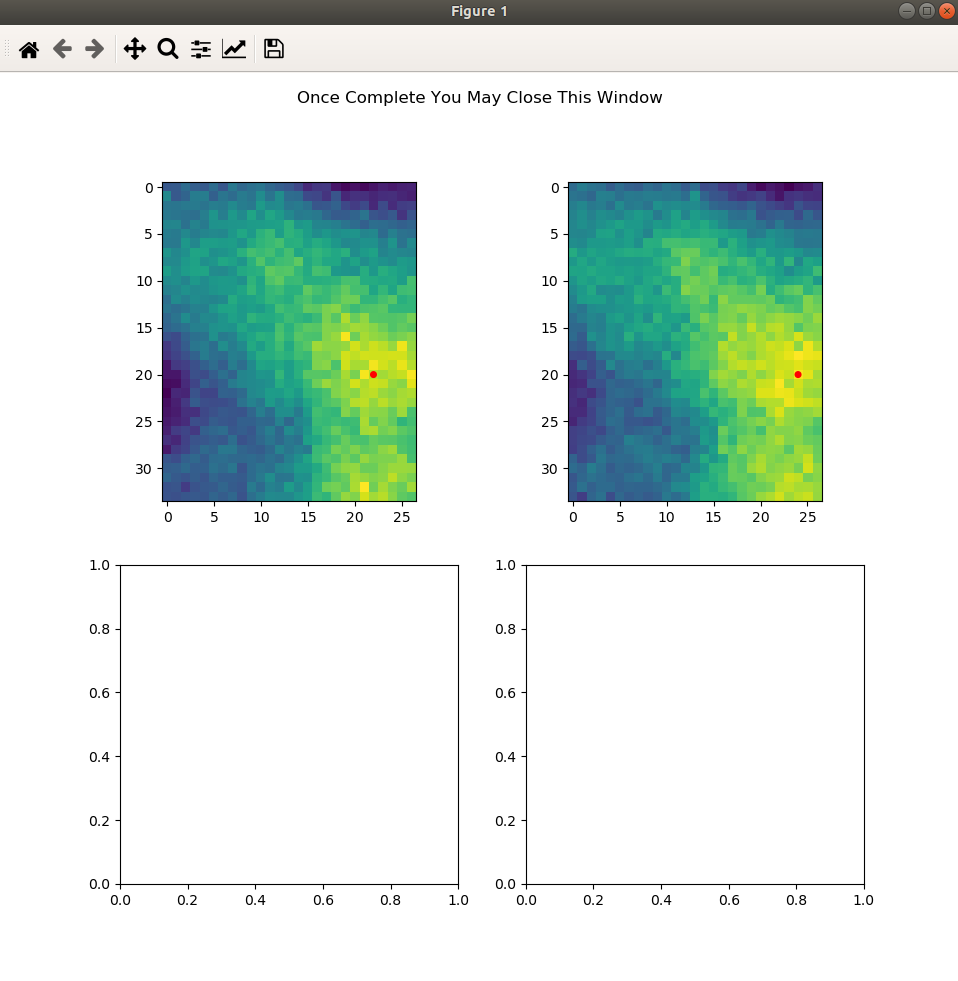
Alignment
In order to acquire reliable spectra, it is important that the frames be aligned properly. Thermal expansion, motor slop, sample damage and imperfect microscope alignment can all cause frames to be misaligned. It is almost always necessary to align the frames before performing any of the subsequent steps.
Aligning the scan can be carried out through the following code and following the GUI. Alignment can only be done of the Fluorescence images or the Region of Interest images set in the setup_det_chan() function. User will define which one to use in the GUI. Once all alignment centers have been set, it is ok to just quit out of the windows.
from sxdm import *
# Select an imported hdf file to use
test_fs = SXDMFrameset(file="...")

# Run through five passes of the default phase correlation
test_fs.alignment(reset=False)
Brings Up All Fluor Maps
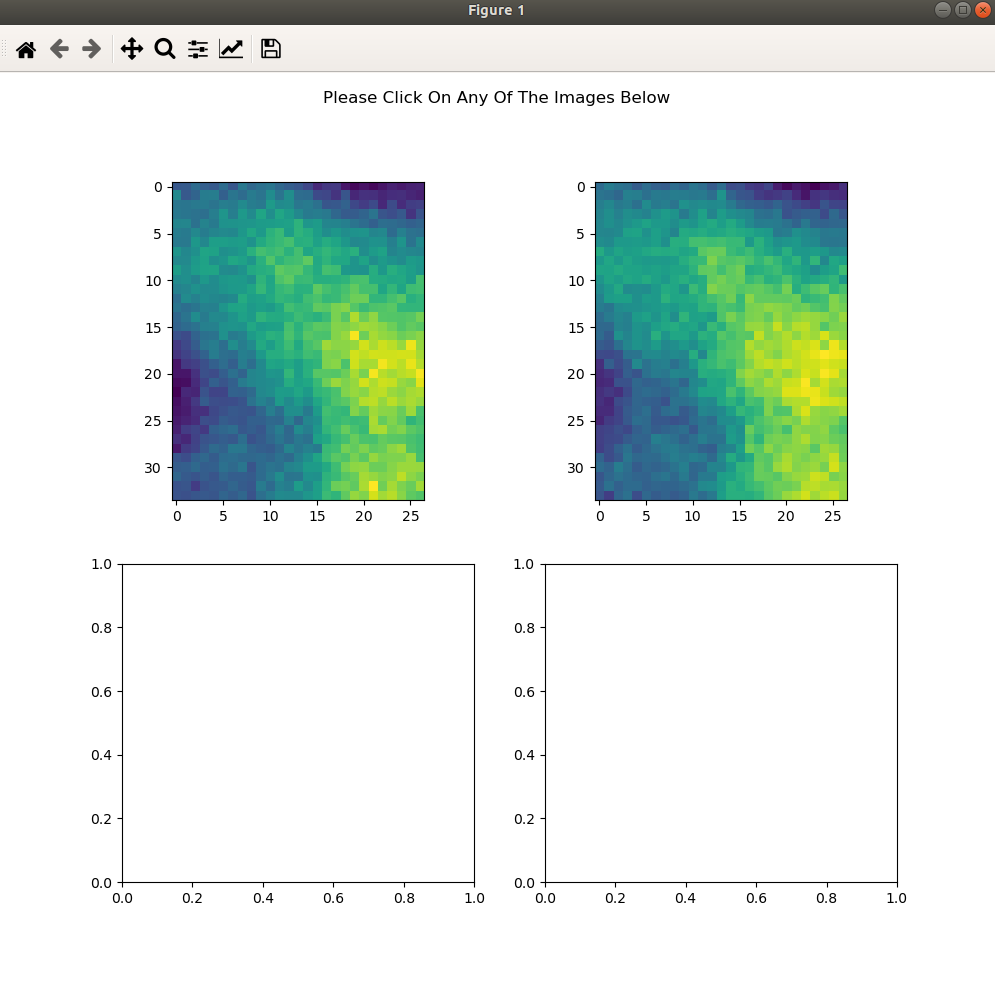
User Select Center
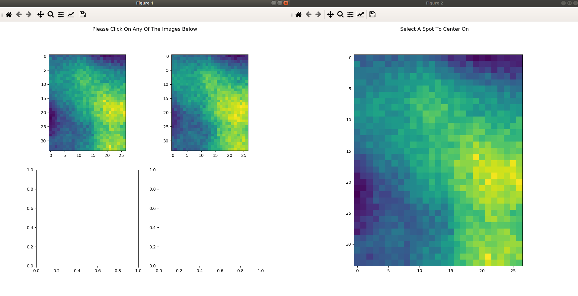
Showing All Centers
reset (bool) - if you would like to completely reset the alignment make this equal True
Note
if you import new scan numbers you must make sure reset=True for the first alignment
Diffraction Axis Values
To determine the chi bounds (angle bounds) for the detector diffraction images as well as determining the numerical aperture, focal length, and instrumental broadening in pixels.
test_fs.chi_determination()
angle difference (in degrees) from the left/bottom hand side of the detector to the right/top test_fs.chi
focal length in millimeters can be called with test_fs.focal_length_mm numberical aperature in millirads can be
called with test_fs.NA_mrads instrumental broadening radius in pixels of the diffraction image can be called with
test_fs.broadening_in_pix
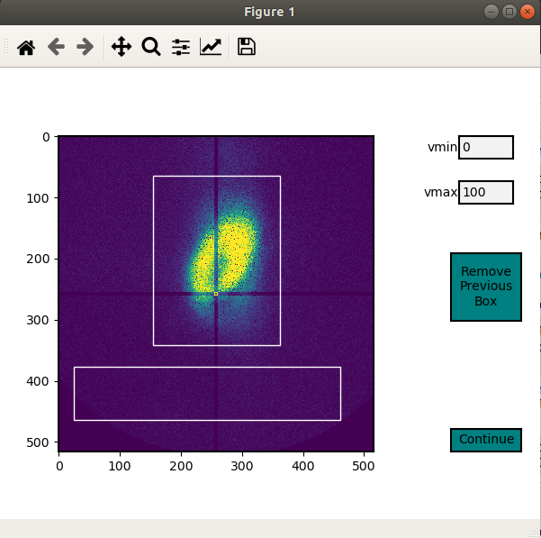
Region Of Interest Analysis
Description
This allows the User to section off multiple areas of the diffraction pattern and create heat maps showing which areas of the Field of View light up these diffraction bounding boxes.
Segmentation
In order for the program to determine a region of interest the User must define areas of interest. This GUI allows the User to define as many Region Of Interests as they please in the diffraction image. Then upon running the Analysis portion, the program will determine the summed value of these regions, plot them, as well as normalize.
Through a GUI the User can select multiple region of interests from the summed diffraction pattern. Set the
diff_segmentation=True in the test_fs.region_of_interest() function for this analysis to be carried out.
# Click and drag on the GUI interface to make roi bounding boxes
test_fs.roi_segmentation(bkg_multiplier=1, restart=False)
bkg_multiplier (int) - an integer value applied to the backgound scans
restart (bool) - if set to True this will reset all the segmentation data
Note
If the program throws image_array doesnt exist run create_imagearray(test_fs)
If the program throws scan_background doesnt exist run scan_background(test_fs)
Analysis
Allows the User to create new ROI maps for all the imported scans in the frameset. This will handle hot and dead pixels as well as show the user the true gaussian distribution of the fields of view.
test_fs.region_of_interest(rows, columns,
                            med_blur_distance=9,
                            med_blur_height=100,
                            bkg_multiplier=1,
                            diff_segmentation=True,
                            slow=False)
rows (int or tuple) - the total amount of rows the User would like to analyze 25 or (10,17)
columns (int or tuple) - the total amount of columns the User would like to analyze 25 or (10,17)
med_blur_distance (odd int) - the chunksize for the median_blur() function
med_blur_height (int) - the amount above the mean to carry out a median blur - selective median_blur option only
bkg_multiplier (int) - the multipler given to the backgound scans
diff_segmentation (bool) - if False the program will skip the segmentation analysis
slow (bool) - defaults to multiprocess data. If the program uses too much RAM the User can set this value to True
to slow down the analysis and save on RAM
To obtain the results from the ROI Analysis use the create_roi() function.
output = create_rois(test_fs.roi_results)
Note
Extremely Large Values??
If the np.nansum(output, axis=(0,1)) values are too high (1e+285) this is due to poor hot pixel removal. Make sure you are using the selective median blur algorithm and lower your median_blur_height value. Also, please see the Viewer section for more details.
Centroid Analysis
Description
This allows the User to determine the diffraction centroid for each pixle in a particular Field of View
Analysis
The centroid analysis function can be called through
test_fs.centroid_analysis(rows,
                            columns,
                            med_blur_distance=9,
                            med_blur_height=10,
                            stdev_min=25,
                            bkg_multiplier=9)
rows - total amount of rows in the scans - can also be a tuple of ints
columns - total amount of columns in the scans - can also be a tuple of ints
med_blur_distance (odd int) - the chunksize for the median_blur() function
med_blur_height (int) - the amount above the mean to carry out a median blur - selective median_blur option only
bkg_multiplier (int) - the multipler given to the backgound scans
stdev_min (int) - the minimum standard deviation of a spectrum which is used to crop signals for centroid determination
slow (bool) - defaults to multiprocess data. If the program uses too much RAM the User can set this value to True
to slow down the analysis and save on RAM
Note
Unsure About Dimension Size
If you are unsure of the dimension sizes call test_fs.frame_shape(). The first number is the number of scans,
the second number is the about of rows + 1, and the third number is the number of columns + 1
Note
Difference Between slow=False and slow=True
The above function calls one of two functions. Either the centroid_pixel_analysis() function and vectorizes it for
moderate run times with excellent RAM management (1-2GB). Or this will call the centroid_pixel_analysis_multi()
function which will multiprocess the dataset, but uses considerably more RAM (6-8GB). Analysis route determine by slow
bool value.
Note
What Is The test_fs.results Variable
Sets the test_fs.results value where the user can return the results of their analysis.
Outputs - [pixel position, zero, median blurred x axis, median blurred y axis, truncated x axis
for centroid finding, x axis centroid value, truncated y axis for centroid finding, y axis centroid value,
summed diffraction intensity]
General User Analysis
Sometimes the built in functions do not align with Users diffraction analysis goals. For this there is a general multiprocessing tool for pixel by pixel diffraction pattern analysis.
Standard Set Up
This creates the User defined frameset
from sxdm import *

test_fs = SXDMFrameset(file'/path/to/file.h5',
            dataset_name='user_dataset_name',
            scan_numbers=[1, 2, 3, 4, ...],
            fill_num=4,
            restart_zoneplate=False,
            median_blur_algorithm='scipy',
            )
Defining a Function
The User will have to define a function that will be applied to the each background corrected diffraction images. If the User would like to perform operations on the Summed Diffraction Pattern please write in summed_dif = np.sum(each_scan_diffraction_post_bk_sub, axis=0) into your first line of your function.
def do_something(each_scan_diffraction_post_bk_sub, inputs):
    """
    each_scan_diffraction_post_bk_sub (preset default)
        - This is an automatic input that has to come first. We are passing in
        - the background corrected diffraction patterns for each test_fs.scan_numbers

    inputs (list of ints, ex. [1, 2, 3, 4])
        - the user defined inputs used to split up into function definitions
        - must be static values

    """

    summed_dif = np.sum(each_scan_diffraction_post_bk_sub, axis=0)

    adding, subtracting, dividing, multiplying = inputs

    first = np.add(summed_diff, adding)
    second = np.subtract(first, subtracting)
    third = np.divide(second, dividing)
    fourth = np.multiply(third, multiplying)

    return fourth, third, second, first

analysis_output = do_something(summed_dif, inputs)
Creating A .tif Image Array
The program needs to have locations for the diffraction.tif images. This creates a centered array for all the locations. The User can choose which scan they would like to center around.
create_imagearray(test_fs)
Implementing General Multiprocessing
This will allow the User to carry out a multiprocesses analysis of the user defined function across all pixels.
# Iterate through the first 10 rows and columns
# OR iterate through rows # - # and columns # - #

rows = 10       # to iterate through row 0 - row 10
# OR  set value to (1, 5) - iterates through row 1 - row 5

columns = 10    # to iterate through col 0 - col 10
# OR  set value to (7, 12) - iterates through col 7 - col 12

inputs = [1, 3, 5, 7]

output = general_analysis_multi(test_fs,
                                rows,
                                columns,
                                do_something,
                                inputs,
                                bkg_multiplier=0)


# The output has a general formula [(row, column), analysis_output]
Conveniently Return General Analysis Values
# Define the analysis outputs: must be in the same order as your original function output
user_acceptable_values = ['fourth', 'third', 'second', 'first']

# Return values
all_values = general_pooled_return(output, 'fourth', user_acceptable_values)

# You can also call 'row_column' or 'help' to show the row and column locations or a list of all acceptable values
# Both 'row_column' and 'help' are created automatically. DO NOT add them to the user_acceptable_values
row_column_values = general_pooled_return(output, 'row_column', user_acceptable_values)
Note
A built in utility checks the computer RAM usage for the User. If the User’s function requires a substantial amount of RAM, the program will default to analysis_output = False. This avoids computer crashes. A warning will also be thrown to the User. To change this value one must go to ~/sxdm/sxdm/generalize.py/general_pixel_analysis_multi and change the 90 in if ram_check() > 90: to the max percent of the computers RAM the User would like to abort analysis at.
Retrieving Imported Data
Return Detector Data - Before Users Set Up SXDMFrameset
scans = [1, 2, 3, 4, 5]
string_scans = scan_num_convert(scans)
return_det(file, string_scans, group='xrf', default=False, dim_correction=False)
Returns all information for a given detector channel for the array of scan numbers.
file - test_fs.file
scan_numbers - test_fs.scan_numbers
group - Examples: filenumber, sample_theta, hybrid_x, hybrid_y, fluor, roi, mis, xrf
default - if True this will default to the first fluorescence image
dim_correction - if True this will add empty rows and columns to smaller datasets to make them the same shape
Return Detector Data - After Users Set Up SXDMFrameset
test_fs = SXDMFrameset(*args)

file = test_fs.file
scan_numbers = test_fs.scan_numbers

return_det(file, scan_numbers, group='fluor', default=False)
Returns all information for a given detector channel for the array of scan numbers.
file - test_fs.file
scan_numbers - test_fs.scan_numbers
group - Examples: filenumber, sample_theta, hybrid_x, hybrid_y, fluor, roi, mis, xrf
default - if True this will default to the first fluorescence image
dim_correction - if True this will add empty rows and columns to smaller datasets to make them the same shape
Centering Detector Data
centering_det(test_fs, group='fluor', center_around=False, summed=False, default=False)
This returns the User defined detector for all scans set in the test_fs.scan_numbers and centers them around a User defined centering scan index
self - the SXDMFrameset
group - a string defining the group value to be returned filenumber, sample_theta, hybrid_x, hybrid_y, fluor, roi
center_around - if this is set to -1, arrays will not be shifted
summed - if True this will return the summed returned detector value (summed accross all scans)
default - if True this will choose the first fluor or first ROI
Note
The centered file numbers are usually stored as test_fs.im_array
Show HDF5 File Groups
h5group_list(file, group_name='base')
This allows the User to view the group names inside the hdf5 file. ‘base’ shows the topmost group. If it errors this means you have hit a dataset and need to call the h5grab_data() function.
file - test_fs.file
group_name - /path/to/group/
Return HDF5 File Data
h5grab_data(file, data_loc)
This will grab the data stored in a group. If it errors this means you are not in a dataset directory inside the hdf5 file.
file - test_fs.file
data_loc - /path/to/data
Show Alignment Data
grab_dxdy(self)
This returns the dx and dy centering values that are stored from the alignment function
self - the SXDMFrameset
Read HDF5 Group Attributes
h5read_attr(file, loc, attribute_name)
This returns the attribute value stored
file - test_fs.file
loc - ‘/path/to/group/with/attribute’
attribute_name - ‘the_attribute_name’
Find Frameset Dimensions
test_fs.frame_shape()
This returns the image dimensions for the SXDMFrameset class object
Calculate Background and FileNumber Locations
test_fs.ims_array()
This will auto load/calculate the background images and the image location array
Show Raw .tif Image Dimensions
test_fs.image_data_dimensions()
This will return the diffraction image dimensions
Pixel Analysis
If the user would like to return a certain pixel analysis value they can use the pixel_analysis_return()
function to achieve this. Returns a dictionary of entries
#'row_column',
#'summed_dif', - auto set to 0 for saving RAM usage
#'ttheta',
#'chi',
#'ttheta_corr',
#'chi_corr',
#'ttheta_cent',
#'chi_cent',
#'roi'
Saving and Reloading Data
Saves self.results to the test_fs.saved_file - this value/file is automatically created in the initial
SXDMFrameset setup
test_fs.save()
To reload saved data in the test_fs.saved_file run
test_fs.reload_save()
This will load the results to test_fs.results